library(cqcr)
library(purrr)
library(dplyr)
#>
#> Attaching package: 'dplyr'
#> The following objects are masked from 'package:stats':
#>
#>     filter, lag
#> The following objects are masked from 'package:base':
#>
#>     intersect, setdiff, setequal, union
library(ggplot2)
library(forcats)
library(tidyr)
CQC Partner Codes
The Care Quality Comission does not require registration or the use
of keys to access the API, but they do want users to attach a partner
code to their requests. If you haven’t been provided a code by the CQC,
you should use a name or acronym that identifies you or your
organisation. You can set the code for each session with
cqc_partner_code(), or store it in an environmental
variable named CQC_PARTNER_CODE.
Using cqcr
Let’s look at the care home options available in a few local authorities in East London. The code below retrieves the ID, name and post code of all care homes in Waltham Forest, Hackney and Tower Hamlets local authorities.
loc1 <- cqc_locations_search(care_home = TRUE,
                             local_authority = c("Waltham Forest",
                                                 "Hackney", "Tower Hamlets"))
Given the list of care home IDs, we can retrieve more detailed
information on each of these locations using
cqc_location_details(). We can use some functions from purrr
and dplyr
to create a data frame with some basic information.
care_home_details <- cqc_location_details(loc1)

care_home_df <- map_dfr(care_home_details, `[`,
                        c("location_id", "name", "number_of_beds",
                          "onspd_longitude", "onspd_latitude"))

care_home_df <- care_home_df %>%
  mutate(rating = care_home_details %>%
           map(c("current_ratings", "overall", "rating")) %>%
           as.character(),
         rating = recode(rating, "NULL" = "No published rating"),
         rating = factor(rating, levels = c("Outstanding", "Good",
                                            "Requires improvement",
                                            "Inadequate",
                                            "No published rating")),
         report_date = care_home_details %>%
           map(c("current_ratings", "reportDate")) %>%
           as.character(),
         report_date = ifelse(report_date == "NULL", NA, report_date),
         specialisms = care_home_details %>% map(c("specialisms", "name")))

care_home_df
#> # A tibble: 193 × 8
#> location_id name number_of_beds onspd_longitude onspd_latitude rating
#> <chr> <chr> <int> <dbl> <dbl> <fct>
#> 1 1-105426344 Checania… 3 -0.0499 51.6 No publ…
#> 2 1-105836127 Forest V… 24 0.00178 51.6 Good
#> 3 1-105885228 Heathlan… 84 0.00269 51.6 Good
#> 4 1-106916349 Aspray H… 64 -0.0169 51.6 Require…
#> 5 1-107269593 Acorn Lo… 98 -0.0533 51.6 Require…
#> 6 1-108969091 St Micha… 11 0.00205 51.6 No publ…
#> 7 1-109015718 Ashcroft… 15 0.0120 51.6 No publ…
#> 8 1-109949478 Rosemead… 20 -0.0141 51.6 No publ…
#> 9 1-110213739 Albany N… 61 -0.0187 51.6 Good
#> 10 1-1105339094 Toby Lod… 10 -0.0401 51.5 Good
#> # … with 183 more rows, and 2 more variables: report_date <chr>,
#> # specialisms <list>Lets take a look at the various specialisms that care homes report. Care homes can report multiple specialisms, so the numbers below add up to more than the number of care homes. I have also used the ratings data to show the number of care homes providing a given specialism with their overall rating.
care_home_df_unnest <- tidyr::unnest(care_home_df, cols = c(specialisms)) %>%
  mutate(specialisms = fct_infreq(specialisms))

theme_set(theme_bw())

p_specialisms_rating <- ggplot(care_home_df_unnest,
                        aes(x = specialisms, fill = rating)) +
  geom_bar() +
  scale_x_discrete(labels = scales::wrap_format(33)) +
  scale_fill_viridis_d(name="", option = "A", end = 0.95) +
  labs(x = "Specialism(s)", y = "Number of Care Homes") +
  theme(legend.position = "bottom",
        axis.text.x = element_text(size = 8, angle = 60, hjust = 1))

p_specialisms_rating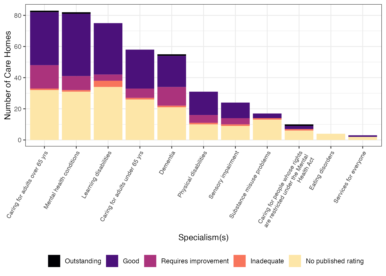
Then, we can map our data with the leaflet
package. In this case the colours indicate the most recent inspection
rating, and the size corresponds to a scaled count of beds.
library(leaflet)

pal <- colorFactor(c("blue", "green", "orange", "red", "gray27"),
                   domain = care_home_df$rating)

labels <- paste0(
  "<strong>Name:</strong> ", care_home_df$name,"</br>",
  "<strong>Number of Beds:</strong> ", care_home_df$number_of_beds, "</br>",
  "<strong>Overall Rating:</strong> ", care_home_df$rating, "</br>",
  "<strong>Report Date:</strong> ", format(as.Date(care_home_df$report_date),
                                           "%e %B %Y"), "</br>",
  "<strong>Specialism(s):</strong><ul><li>",
  lapply(care_home_df$specialisms, paste, collapse='</li><li>'), "</li></ul>"
) %>% lapply(htmltools::HTML)

map <- leaflet(care_home_df) %>%
  addTiles() %>%
    addCircleMarkers(lng = ~onspd_longitude,
             lat = ~onspd_latitude,
             label = labels,
             color = ~pal(rating),
             radius = ~scales::rescale(care_home_df$number_of_beds, to = c(5, 15)))

map